
Pareto Task Inference (ParTI) method
Purpose and context
polytope a geometric object with flat sides
simplex the generalization of triangles (2D) and tetrahedrons (3D) to n dimensions
archetype a combination of traits that yields optimal performance at a given task
Pareto front combination of traits that cannot be improved at a task without diminishing performance at another task
Biological research increasingly depends on interpreting large datasets in high dimensional space. The main approaches for analyzing such data are dimensionality reduction techniques such as principal component analysis, and clustering techniques that split data points into groups. Recently, a theoretical advance (Shoval et al., Science 2012) has suggested a complementary way to understand large biological datasets. This approach is based on Pareto optimality of organisms with respect to multiple evolutionary tasks. It predicts that cells or organisms that need to perform multiple tasks have phenotypes that fall on low dimensional polytopes such as lines, triangles, tetrahedrons; phenotypes optimal for each task – called archetypes – are at the vertices of these polytopes. This idea has so far found applications in fields such as ecology (Sheftel at al., 2013; Szekely et al., 2015; Tendler et al., 2015), evolution and development (Kavanagh et al., 2013), biological circuit design (Szekely et al., 2013) and gene expression analysis of cell populations (Hart et al., 2015) and single cells (Korem et al. 2015, Adler et.al 2019).
An introduction to Pareto optimality in evolution is available here.
The present page offers a software package that implements the Pareto Task Inference (ParTI) method to analyze biological data in light of Pareto theory. ParTI finds the best fit polytopes and the corresponding archetypes and indicates which features of the data are enriched near each archetype. The present approach is less sensitive to the density of sampling of the data space than clustering approaches because it relies on the overall shape of the data and its pointy vertices; enrichment of relevant biological features is higher near the archetypes than near the centers of clusters obtained by standard methods.
The package comes with two example datasets and template scripts to analyse them: a dataset of 2000 tumor breast cancer gene expression dataset by Curtis et al., Nature 486, 345 (2012), and 63 mouse tissues by Lattin et al., Immunome Res 4, 5 (2008).
The concepts used in the package are introduced in its accompagning manuscript and in the manual:
- Main text and Supplementary material
- Supplementary figure: rotatable breast cancer dataset (Mathematica figure)
- Manual
- Caveats
We strongly recommend getting familiar with these concepts by reading the manuscript (30-60min) and going over the manual (20min) before using the software package.
While programmers and developers can follow the latest developpments of the package on GitHub, we encourage normal users to download the stable version of the package.
Credits
The software package includes 5 algorithms to find the position of the archetypes from high-dimensional data, developped by other authors for other purposes (e.g. remote sensing). We integrated them in ParTI to save the user the burden of downloading, installing and configuring the different algorithms, which include:
- Sisal by Bioucas-Dias JM, “A variable splitting augmented lagragian approach to linear spectral unmixing,” in Proc. IEEE GRSS Workshop Hyperspectral Image Signal Process.: Evolution in Remote Sens. (WHISPERS), 2009, pp. 1–4.
- MVSA by Li J and Bioucas-Dias JM, “Minimum volume simplex analysis: A fast algorithm to unmix hyperspectral data,” in Proc. IEEE Int. Conf. Geosci. Remote Sens. (IGARSS), 2008, vol. 3, pp. 250–253.
- MVES by Chan T-H, Chi C-Y, Huang Y-M and Ma W-K, “Convex analysis based minimum-volume enclosing simplex algorithm for hyperspectral unmixing,” IEEE Trans. Signal Process., vol. 57, no. 11, pp. 4418–4432, 2009.
- SDVMM by Chan T-H, Ambikapathi A, Ma W-K and Chi C-Y, “Fast algorithms for robust hyperspectral endmember extraction based on worst-case simplex volume maximization,” in IEEE International Conference on Acoustics, Speech, and Signal Processing (ICASSP), 2012.
- PCHA by Mørup, M. & Hansen, L.K, "Archetypal analysis for machine learning and data mining", in Neurocomputing 80, 54–63 (2012).
Guide to using the ParTI package
Installation in 3 steps
You will need Matlab pre-installed on Linux or Windows. The package also runs on Mac OS X, but some minimal polygon finding algorithms (among which MVES and MVSA) currently do not work on this platform.
- Download the Matlab software package implementing the method (last update: Jan 26th 2020).
- Uncompress the archive.
- Start Matlab from within the particode/ directory.
Quick start
For a quick start, open and run the script exampleSynthetic.m for a rapid feel of ParTI on a small synthetic dataset with just one property per data point.
Then, consider the exampleCancer.m, exampleCancerRNAseq.m and exampleMouse.m, which respectively load and analyze the datasets of Curtis et al., RNAseq profiles of TCGA breast cancer tumors, and Lattin et al. featured in the article.
These three templates come with in-code documentation and can be adapted to analyse other datasets.
Passing your dataset to ParTI
Alternatively, you can write your own pipeline to load a dataset into Matlab and prepare it for the analysis. Then run ParTI by calling one of the two master functions of the package, ParTI_lite() and ParTI(), which are respectively located in the ParTI.m and ParTI_lite.m files.
Contrary to ParTI(), ParTI_lite() does not compute the p-value of the identified polytopes nor errors on the archetypes which require to repeatedly reshuffle the dataset. This leads to a dramatic increase in speed: in the case of the cancer data of Curtis et al., Nature (2012) supplied with the package, the entire analysis can be performed in a few minutes with ParTI_lite(), while the complete statistical assessment performed by ParTI() may require several hours for large datasets (e.g. 4h for the cancer data of Curtis al. on a 3.4GHz CPU with 8 GB of RAM on Matlab 2013). Therefore, we recommend to first explore new data sets using ParTI_lite(), and then confirm the statistical significance of the findings using ParTI().
The ParTI_lite() and ParTI() functions require the following parameters, all of which are optional except for the first one (dataset):
- DataPoints, a matrix with the values of different traits (the coordinates, e.g. expression level of genes). Each sample is a row, each trait (e.g. each gene) is a column. We recommend log-transforming gene expression data (e.g. log-mRNA abundance or log-fold change) prior to analysis with ParTI.
- algNum choses the algorithm to find the simplex: 1 for Sisal (the default), 2 for MVSA, 3 for MVES, 4 for SDVMM, 5 for PCHA. If the dataset features a large number of data points, Sisal is recommended. In our experience, a large number of points means at least 10 per dimension (after dimension reduction): 10 points in 1D, 100 points in 2D, 1000 points in 3D, etc.. If a smaller number of data points is provided, MVSA should be preferred.
- dim, the dimension up to which dimension the Explained Variance (EV) should be calculated. EV is defined as the average distance between the data points and the best simplex defined by the archetypes found by PCHA. We recommend to start with a dimension between 5 - 10, and increase the dimension until an inflexion be spotted the EV curve. Default value is set to 10.
- DiscFeatName, a list of the Discrete Feature labels, as a row vector. Default value is an empty list. An empty list can be used as input if no discrete features exist.
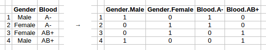
- EnMatDis, a boolean matrix or a string cell array in which columns represent discrete feature and rows represent datapoints. For instance, if the data being analyzed is gene expression levels across many patients, DataPoints (see first parameter) is a matrix with patients as rows and genes as columns. EnMatDis would then be a matrix with patients as rows and discrete clinical attributes of each patient as column: gender, blood type, ethnicity, etc.. Note that the ordering of rows in the datapoints matrix should match that of EnMatDis. Similarly, the ordering of the columns in EnMatDis should reflech that of DiscFeatName. Default value is an empty list. An empty list can be used as input if no discrete features exist.
- cols, the index of the columns of EnMatDis to booleanize, if EnMatDis is a string cell array rather than a boolean matrix. To booleanize all columns, set to 0. Default value is an empty list. An empty list can be used as input if no discrete features need to be booleanized. The table on the left hand side below shows the matrix before booleanization, while the table on the right side shows the table after booleanization:
- ContFeatName, a list of the Continuous Feature labels, as a row vector. Default value is an empty list. An empty list can be used as input if no continuous features exist.
- EnMatCont, a real matrix in which columns represent continuous attributes and rows represent datapoint attributes. For instance, if the data being analyzed is gene expression levels across many patients, DataPoints (see first parameter) is a matrix with patients as rows and genes as columns. EnMatCont would then be a matrix with patients as rows and discrete clinical attributes of each patient as column: blood pressure, body-mass index, age, etc.. The ordering of the rows should match those in EnMatCont while the ordering of the columns should match those in ContFeatName. Default value is an empty list. An empty list can be used as input if no continuous features exist.
- GOcat2Genes, a boolean matrix of genes x continuous features which indiciates, for each continuous feature, which genes are used to compute the feature. It is used in the leave-one-out analysis carried out by ParTI() and ignored by ParTI_lite(). The MakeGOMatrix() function can be used to compute this matrix. Default value is an empty list.
- binSize, the fraction of the datapoints that should be grouped in a single bin when calculating feature enrichments. The article that introduces the method proposes a principled way to determine how to set this number (see supplementary material). In our experience, setting the binSize in such way that 10 - 100 points end up in each bin appears to be a reasonble practice. For instance, for a dataset with ~60 points, a binSize of 0.2 would yield 60 x 0.2 = 12 points per bin. Similarly, for a dataset with ~2000 points, a binSize of 0.05 would yield 2000 x 0.05 = 100 points per bin. Default value is 0.05.
- OutputFileName, a prefix that will be used to name the Comma Separated Files (CSV) to save the results of the enrichment analysis. For instance, setting this parameter to 'Cancer_' will create four CSV spreadsheets named Cancer_enrichmentAnalysis_continuous_All.csv, Cancer_enrichmentAnalysis_continuous_significant.csv, Cancer_enrichmentAnalysis_discrete_All.csv and Cancer_enrichmentAnalysis_discrete_significant.csv. These spreadsheet summarize the enrichment analysis for discrete and continuous tables, with and without filtering out non-significant attributes. Default value is 'ParTIoutputFile'.
Output of the ParTI analysis
Upon completion, the ParTI() function returns the following Matlab output:
- arc, the coordinate of the archetypes in the space spanned by the principle components.
- arcOrig, the coordinate of the archetypes in the original space, defined by datapoints.
- pc is a double matrix that saves the projected dataset in the lower dimensional space spanned by the principal components.
- errs, the covariance matrix of the uncertainty on the archetypes. Estimated by bootstrapping. Only ParTI() will return this output.
- pval, the p-value that the dataset is described by a simplex. Only ParTI() will return this output.
In addition, the function creates the following figures and tables:
- the function creates CSV tables summarizing the enrichment analysis for discrete and continuous tables. CSV files whose names end in ...significant.csv contain only features that are significantly enriched close to archetypes whearas files whose names end with ...All.csv have enrichment statistics for all features at all archetypes. Each row in the .csv files represent a feature. First column is the archetype number, second column is the feature name, 3rd column represents the p-value that the feature is enriched near the mentioned arcehtype, 4th column indicates whether the feature is significant after controling to multiple-hypthesis testing (1 - significant, 0 - not significant), and the 5th column indicates Pmax - the probablity that the enrichment of the feature is maximal near the archetype (in the lite version this column is 1 if the enrichent at the closest bin is maximal and 0 otherwise). The lower the p-value and the higher Pmax, the stronger the feature is correlated with the archetype. The features that appear in the "significant" file can be used to infer the biological tasks of each archetype.
- explained variance by each principal component. This figure lets you determine how many dimensions are necessary to describe the dataset. For instance, the knick in the curve below suggests 3 dimensions.

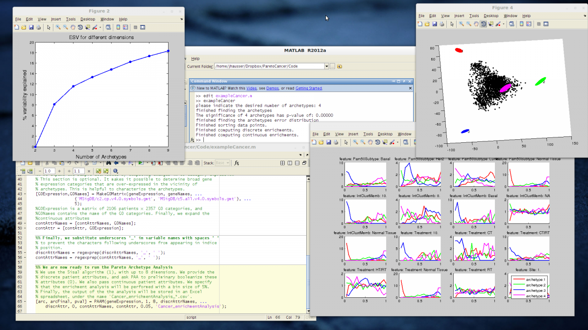
- Explained Sample Variance (ESV) curve to set the number of archetypes. For example, on the figure below, increasing the numbers of archetypes past 4 yields little improvement in terms of explained sample variance. A good choice might hence be 4 archetypes.

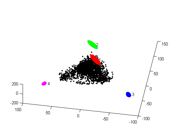
- 2D and a 3D figure showing the position of the archetypes relative to the data

- enrichment curves, which show how the enrichment in different attributes changes as one moves away from the archetypes. For example, in the figure below, we see that normal tissues are strongly enriched close to archetype 4 while samples of the LumB PAM50 subtype are maximally enriched close to archetype 1.


Frequently asked questions
What are the differences between the different algorithms, what are their pros/cons?
- Sisal: Minimizes the volume of the simplex that encapsulates the data. It is resilient to noise and outliers - data points can end outside of the simplex. Usually archetype are located outside the data. (default)
- MVSA/MVES: Minimizes the volume of the simplex that encapsulates the data. It is not resilient to noise and outliers - data points will all be inside the simplex.
- SDVMM: data points are selected as archetypes, maximizing the variance of the data encapsulated within the resulting simplex. By Selecting tolerance radius around the points selected as archetypes, one can expand the simplex. In general, the archetypes are located within the data.
- PCHA: archetypes are found within the convex hull of the data, maximizing the data encapsulated within the resulting simplex. By selecting a tolerance radius around the points selected as archetypes, one can expand the simplex. In general, the archetypes are located within the data.
For large datasets of thousands data points, the three minimal bounding simplex algorithms (SISAL, MVSA and MVES) give very similar results. We found that the SISAL algorithm performs best since it takes good care of outliers in the dataset and gives the tightest simplex enclosing most of the data points. It is then also natural to use SISAL for calculation of the simplex statistical significance.
However, when the number of data points is on the order of a hundred or less, the SISAL algorithm might ignore important points when calculating the enclosing simplex. This is most relevant when calculating the statistical significance of the simplex. In such cases we used the MVSA algorithm.