Sparsity Constrained Nonlinear Optimization

A. Beck and Yonina C. Eldar

Introduction

Sparsity has long been exploited in signal processing, applied mathematics, statistics and computer science for tasks such as compression, denoising, model selection, image processing and more.
Here we consider recovering a sparse vector from nonlinear measurements. More generally, we treat the problem

min ƒ(x) s.t. ||x||₀ ≤ k

where

ƒ(x) is an arbitrary continuously differentiable function
Not necessarily convex!

We present and analyze several different optimality criteria which are based on the notions of stationarity and coordinate-wise optimality. These conditions are then used to derive three numerical algorithms aimed at finding points satisfying the resulting optimality criteria: the iterative hard thresholding method and the greedy and partial sparse-simplex methods. The first algorithm is essentially a gradient projection method while the remaining two algorithms extend the popular orthogonal matching pursuit algorithm to the nonlinear setting. Theoretical convergence of these techniques and their relations to the derived optimality conditions are studied.

A special case is the Phase retrieval problem in which

$" "$

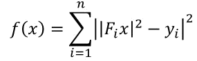
where F_i is the ith row of the Fourier matrix. For details on this problem see phase retrieval page .

The IHT Method

A well-known solution method is the so-called iterative hard-thresholding (IHT) method whose recursive update formula is

$" "$

The Greedy Sparse-Simplex Method

The next method is an extension of orthogonal matching pursuit (OMP) to the nonlinear setting. It is shown to converge to a coordinate-wise minimia, which is a stronger optimality then L-stationarity. Thus, this approach tends to perform better than IHT and works under more relaxed conditions.
To invoke the greedy sparse-simplex method, two MATLAB functions should be constructed. The first one is the objective function and the second is a function that performs one-dimensional optimization with respect to each of the coordinates and outputs the index of the variable causing the largest decrease, its optimal value and the corresponding objective function value. For the least squares problem the MATLAB function is in f_LI.m and the second required function is g_LI.m.
After having these two functions, we can now invoke the main function greedy_sparse_simplex.m.

The Partial Sparse-Simplex Method

The partial sparse-simplex method is implemented in the m-file partial_sparse_simplex.m. The input arguments are the same as the one of greedy_sparse_simplex expect for one additional input argument which is the gradient function. For the function f_QU, the gradient is implemented in the m-file gradient_QU.m.

Reference

A. Beck and Y. C. Eldar, "Sparsity Constrained Nonlinear Optimization: Optimality Conditions and Algorithms", SIAM Optimization, vol. 23, issue 3, pp. 1480-1509, Oct. 2013.

Software Download

Download Sparse-Simple Matlab Package.

Installation:
1. Unzip all files to a directory of your choice.
2. Open guide.pdf file and follow the steps.